First of all, look at what's called "carlman." like other well-known theories (e. G. Fourier, taylor, etc.), kalman is a human name, but unlike them, he is a modern man!
1. Rudolf emil kalman
Hungarian mathematician born in 1930 in budapest, the capital of hungary. 1953, obtained b. A. And m. A. Degrees in electrical engineering at mit in 1954. Doctorate, columbia university, 1957. The kalman filter that we are now studying stems from his doctoral dissertation and his 1960 paper, a new approach to linear filtering and production products (the new method of linear filtering and prediction issues)。
In short, the kalman filter is a “optimal recursive data processing algorithm”. He is the best, the most efficient, and even the most useful, to solve most of the problems. His extensive applications have been in place for over 30 years, including robots, human navigation, control, sensor data integration, even military radar systems and missile tracking. In recent years, they have been more applied to computer image processing, such as head-face recognition, image fragmentation, image edge detection, etc。
Introduction to the kalman filter
In order to understand the kalman filter more easily, images are used to describe it, rather than listing a whole array of mathematical formulas and mathematical symbols, as is the case in most reference books. But his five formulas are at the heart of it. Combining modern computers, the kalman program is quite simple, as long as you understand his five formulas。
Before introducing his five formulas, let us explore them step by step, based on the following example。
Suppose we're going to study the temperature of a room. According to your experience, the temperature of this room is constant, that is, the temperature of the next minute equals the temperature of the present minute. Let's say we'll take a minute to do the unit. Assuming you're not 100% convinced of your experience, there might be some deviations. We see these deviations as white gaussian noise, which is that they are irrelevant and consistent with gaussian distribution. Also, we put a thermometer in the room, but the thermometer is not accurate, and the measurements will differ from the actual values. We also see these deviations as gaussian noise。
Now, for a minute we have two temperature values for the room: your experience-based projection (systemic projection) and the thermometer (measurement). We're going to use these two values, combined with their respective noises, to estimate the actual temperature of the room。
If we're going to estimate the actual temperature at k-hours. First of all, you have to predict the temperature at the k-1 time. Because you believe the temperature is constant, you'll get the k-hour temperature projection at the same time as k-1, assuming 23 degrees, and at the same time the goss noise deviation of the value is 5 degrees. If the deviation of the best temperature values estimated at the k-1 time is 3 and you're not sure about your own projections is 4 degrees, they're squared and squared, which is 5. And then you get the k-hour temperature from the thermometer, assuming it's 25 degrees, and the deviation is 4 degrees。
Because we estimate the actual temperature at k-hours with two temperature values, 23 and 25 degrees, respectively. What's the actual temperature? Believe yourself or believe in thermometers? We can judge who believes more. Because kg^2 = 5^2/(5^2+4^2), kg=0. 78, we can estimate the actual temperature at k-time at 23+0. 78* (25-23) = 24. 56 degrees. As can be seen, the best temperature values are calculated in favour of thermometers because the thermometers are relatively small (more believed in thermometers)。
Now we've got the best temperature at the k-hour, and the next step is to get to the k-plus-one and make new best estimates. So far, nothing seems to have come back. By the way, before we go into k+1, we have to calculate the deviation of the best value (24. 56 degrees) at k-time. The algorithm is as follows: ((1-kg)*5^2) ^0. 5=2. 35. The five here is the deviation of the 23 degree temperature values you predicted at the k-point above, and the resulting 2. 35 is the deviation of the best temperature values estimated at the k-point after the k-point (equivalent to 3 above)。
This is how the calman filter constantly returns the covariance, thus estimating the best temperature values. He's running fast, and it only kept a moment's covariance. The kg above is kalman gain. Isn't it amazing that he can change his worth at different times!
Here's what we're going to do. We're going to talk about kalman on the real engineering system。
3 the kalman filter algorithm
In this section, we come to describe the kalman filter that originated in dr kalman. The following description would cover some basic conceptual knowledge, including probability, and the immediate variables (random variable), gaussian distribution, and state-space mode. But the details of the kalman filter cannot be described here。
First, we need to introduce a system of discrete control. The system can be described as a linear random differential equation:
X(k)=ax(k-1)+b u(k)+w(k)
Plus systematic measurements:
Z(k)=hx(k)+v(k)
In the previous two subs, x(k) is a k-hour system state and u(k) is a k-time control of the system. A and b are system parameters, and for multi-model systems they are matrices. Z(k) is the measurement of k-hours, h is the parameter of the measurement system and h is the matrix for the multiple measurement system. W(k) and v(k) indicate process and measured noise, respectively. They're assumed to be white gaussian noise, and their covariance is q, r。
Calman filters are the best information processor for meeting the conditions above (the linear random differential system, both process and measurement are gaussian white noise). We're going to use them to estimate the optimal output of the system with their covariances。
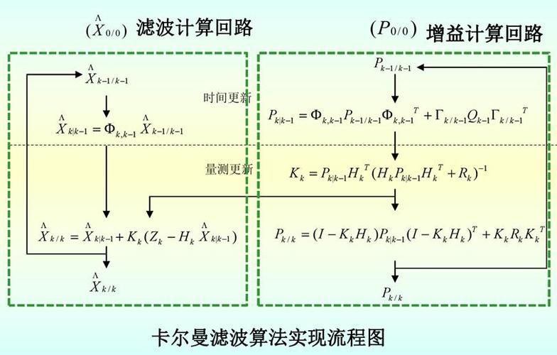
First, we're going to use the system process model to predict the next state of the system. Assuming that the current system state is k, based on the system model it is possible to predict a state based on the previous state of the system:
X(k|k-1) = ax(k-1|k-1) +b u(k) (1)
In formula (1), x(k|k-1) is the result of a projection using the previous state, x(k-1|k-1) is the best result of the previous state, u(k) is the control of the present state and, if not, it can be zero。
So far, our system results have been updated, but the covariance corresponding to x (k|k-1) has not been updated. We use p for covariance:
P(k|k-1) = ap(k-1|k-1) a'+q (2)
In formula (2), p (k|k-1) is the covariance corresponding to x (k|k-1), p (k-1|k-1) is the covariance corresponding to x (k-1|k-1), a ' indicates that a is the transition matrix and q is the covariance of the system process. The first two of the five formulas of the kalman filter, i. E. The prediction of the system。
Now we have the results of the current state, and then we collect the measurements of the present state. When combined with projections and measurements, we can obtain the optimal estimate of state (k) x (k|k):
X(k|k) = x(k|k-1) + kg(k) (z(k)-hx(k|k-1)) (3)
Kg is kalman gain:
Kg(k) = p(k|k-1) h ' / (hp(k|k-1) h ' + r) (4)
So far, we've got the best estimate under k state x (k|k). But in order to keep the kalman filter running until the end of the system, we also need to update the covariance in k(k|k):
P(k|k)=(i-kg(k)h)p(k|k-1) (5)
Of these, the matrix i is 1 is measured for single model sheets, i = 1. When the system enters k+1, p(k|k) is the p(k-1|k-1) of the formula (2). So the algorithm can go back to the operation。
The principles of the kalman filter are basically described, and formulas 1, 2, 3, 4 and 5 are his five basic formulas. Under these five formulas, computer programs can be easily achieved。
I'll use the program to give an example。
4 simple example (a simple example)
Here, in conjunction with section ii, we give a very simple example of the work of the kalman filter. The example given is a further description of section ii and will be accompanied by a programme simulation。
As described in section ii, the room is seen as a system, which is then modelled. Of course, the models we see need not be very precise. All we know about this room is at the same temperature as at the previous moment, so a = 1. No control, so u(k)=0. It follows:
X(k|k-1) = x(k-1|k-1) (6)
The formula (2) could be replaced by:
P(k|k-1) = p(k-1|k-1) +q (7)
Because the values measured are thermometers, which correspond to the temperature, h=1. Model 3,4,5 could be replaced by the following:
X(k|k) = x(k|k-1) + kg(k) (z(k)-x(k|k-1)) (8)
Kg(k) = p(k|k-1) / (p(k|k-1) + r) (9)
P(k|k) = (1-kg(k)) p(k|k-1) (10)
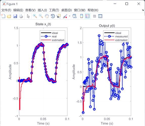
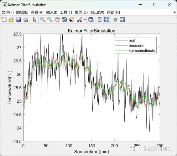
Now we simulate a set of measurements as input. Assuming that the real temperature of the room is 25 degrees, i simulated 200 measurements with an average of 25 degrees, but added a few degrees of hyper-white noise (the blue line in the chart)。
In order for the kalman filter to start work, we need to tell kalman the initial values for the two moments, x (0|0) and p (0|0). They don't care much about their value, just give one, because with kahrman's work, x will gradually shrink. For p, however, it is generally not possible to take zero, because this might give kalman full confidence that your x (0|0) is the best in the system, so that the algorithm cannot be reduced. I chose x (0°) = 1 degree, p (0°0) = 10。
The true temperature of the system is 25 degrees, which is shown in the figure by black wire. The red line in the graph is the optimal result of the calman filter output. The result is set in algorithm q=1e-6, r=1e-1)。
Xxxxxxxxxxxxxxxxxxxxxxxxxxxxxxxxx
A kalman filter under matlab:
Okay, clear
N = 200;
W(1) = 0;
W=randn (1,n)
X(1) = 0;
A = 1;
For k=2:n;
X(k)=a*x(k-1)+w(k-1);