One, what's a kalman filter
Kalman filtering is an algorithm that provides the best estimate of the state of the system by using linear system state equations through system input and output observations. As observations include the effects of noise and interference in the system, the best estimate can also be considered as a filtering process。
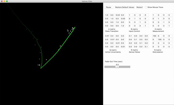
It's like moving a target in motion, and every moment there's "where is it actually going" and "how fast is it going" -- these real states. But the sniper does not see these "real values" and can only get observations with errors through the lens (sensor) (e. G., "like 100 metres, possibly half a metre to the left"。
"noise and interference" in observational data, like leaves, fog, tree cover in front of the lens
When the leaves block the sight (observation data suddenly do not), the kalman filter does not fully believe in the frame, but relies more on “predicts based on target motion patterns” (e. G., “the target just ran at a flat speed, it was impossible to jump 10 meters suddenly, the frame data must have been blocked by the leaves and ignored”)。
When the sight is clear (observation is reliable), filters modify the pre-observation with new observations (e. G., "successfully 105 meters, like i thought, just a little bit of the point of view."。

Kalman filters are like an experienced sniper: prejudiced by target motion patterns (system models), modified by noise-based observations (sensor data), and eventually locked in the interference. This process neither blindly believes in single observations (filtration of noise) nor persists in relying on historical judgement (in combination with new information) to achieve “best estimates”。
2 extension of ekf and kf
The original application of kalman's filtering theory to only linear systems, bucy, sunahara and others proposed and studied the expansion of the kalman filter (extended kalman filter, ekf) to further apply the kalman filtering theory to non-linear areas. The basic idea of the ekf is to linearize the non-linear system and then conduct the kalman filter, so the ekf is a suboptimal filter. Since then, the introduction and application of a wide range of second-order kalman filters has further enhanced the estimation of kalman filters for non-linear systems. The secondary filtering method, which takes into account the secondary subdivisions of the taylor tier, reduces the estimated error due to linearization, but increases the amount of the operation substantially, so that there is no one-step ekf application in practice。
The full name of ekf is extended kalmanfilter, which is an extended kalman filter, an efficient re-entry filter。
The expansion of the ekf is an “upgraded version” of the kalman filter, designed to address the uncertainty of the kalman filter. We can continue to understand their relationship using the metaphor of "snipers aim at moving targets":
Kalman filter (kf): can only deal with “procedural objectives”
The core premise of the kalman filter is that the target's pattern is “linear”。
For example, a moving target moves in a flat-speed straight line (almost at the same speed and direction) or a flat-speed motion (one m/s per second) -- these movements can be described in simple linear formulas (e. G. "next-second position = current position + speed x time")。
At this point, snipers can predict with a flat speed / flat acceleration model, and kalman filter formulas can be applied directly, calculating simple and efficient。
Expansion of the kalman filter (ekf): to address the “defunct targets”
But in reality, the movement of many targets is "non-linear":
And that's when kalman filters don't work -- because its formula can only deal with linear relationships, and in the face of the turning target, it's going to be more and more different with the "spacing straight line" model。
The effect of ekf is to turn non-linear problems into linear:
It uses a non-linear motion track (like a curve aggregating with many small lines) near the "current estimated status point". So we can continue to use the linear formula of the kalman filter, but we have to recalculate the "cutter line" every time。
Summarizing: relationships are like the foundation calculator and the scientific calculator
3 and ekf integration of imu and odom calculations
We can imagine the integration of the ekf with the imu and the odom as a game of "guessing positions," and you need to combine the two "closes" to constantly correct your guess and make the results more accurate。
Imu and odom are very important concepts in the robotic field and in other systems involving motion perception and positioning, as detailed below:
Imu (inertial measurement unit)
Odom (mileometer)
Let's make a simple picture of two thread sources:
Ekf does this by using the imu's "real-time feeling" to guess first, then the odom's "roadmark information" to fix it, and finally to get a quick and accurate result. In two steps:
Step 1: use of imu “guidance” (projection phase)
Suppose you're going to walk to the supermarket now, ekf first guess your position and speed per second based on imu information. For example:
But the ekf knew that the imu would "run out," so the guess left a "fault range": for example, "it's about 1 metre, and the error could be 0. 5 meters." (this error will grow as much as the imu uses it, as if the guess is getting worse and worse.)。
Step 2: use of odom "amendment" (update phase)
And for a while, odom, this "roadmark," said, "by the number of wheel circles, you're going to be `1. 2 meters from the door of the district."。
It's time for ekf to do two things:
For example:
The correction will also reduce the margin of error (e. G. From 0. 5 m to 0. 2 m), as the two threads cross-check and the result becomes more specious。
It's going back and forth. It's getting better and better
Then i repeat these two steps:
In this way, both the advantage of the imu “fast reaction” (real time and tight motion) and the advantage of the odom “no bias” (correcting cumulative error) are used, and the final position, speed and accuracy are obtained。
In short, ekf is like a "smart judge":
4. A dark and incomprehensible projection formula
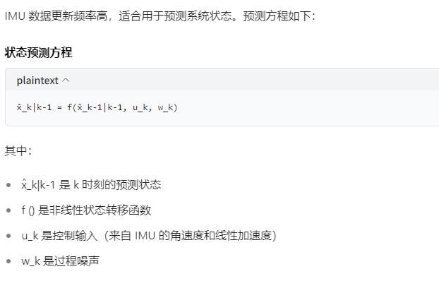
This equation is the core predictive equation that expands the ekf. It's really abstract. I'll explain it step by step and make it easier to understand。
Intuitive understanding of the state prediction equation
This equation describes how the current state of the system is projected on the basis of estimates of the state of the previous moment and current control input。
We can use an example of life:
State of the previous moment: just as you now know your location and speed
Control input: like you know you're moving forward or turning around
Prognosis: on the basis of current location, speed and movement, predict where you will be at the next moment
Mathematical symbols explain in detail
Let's break this equation:
Symbolic meaning:
F(): this is a function indicating how the state moves from one moment to the next
U k: control of input, e. G. Acceleration and angle speed of imu measurements
W k: process noise, indicating system uncertainty (e. G., your actions may not be fully implemented as planned)
More specific examples: mobile robots
Assuming we have a robot moving on the plane, its state includes:
Summary
The core idea of the state projection equation x|k-1 = f (x̂k-1|k-1, u k, w k) is:
Through this equation, ekf is able to predict changes in the system's state using high frequency input data such as imu。
5. Process noise coordination matrix
Process noise arrange matrix
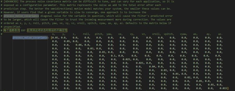
Matrix structure to state
The rows and columns of the matrix strictly correspond to the order of the ekf status vector, usually:
Oh, yeah, yeah, yeah, yeah, yeah
Each element
Meaning:
2. Line-by-line / column reading (using your configuration as an example)
Below is an explanation of the physical significance of the diagonal elements (which are mostly zeros, representing the independence of noise), combined with the common robotic motion scene (e. G. Differential chassis, mechanical arm):
State dimensions
Index
Diagonal value
Meaning (uncertainty in projections)
Location
0. 05
The presumed noise intensity (e. G. Robots moving on x-axis, position deviation due to model error is "like this" when predicting x-direction position
0. 05
Y prognosis of position
0. 06
Z predicted noise at directional position (altitude) (lower noise if robots are terrestrial mobile devices,z less change; larger if flight involved)
Attitude (angles)
# roll #
0. 03
Prognostic noise (e. G., model assumption of “change of attitude”, but actual error due to vibration, etc.)
I don't know
0. 03
Pitch's predicted noise
Yaw
0. 1
The predicted noise of the deviant angle (yaw when the ground robot turns, yaw is vulnerable to interference, noise is usually greater)
Line speed
Vx
0. 025
X predicted noise at the speed of the direction line (model assumed "pace " , but actual deceleration and slippage would cause error)
Vy
0. 025
Y noise projected for directional speed
Vz
0. 04
Z predicted noise at direction line speed (high rate of change)
Angular speed
Volll
0. 01
The projected noise of the rolling angle speed
Vpitch
0. 01
The predicted noise at the altitude
Vyaw
0. 02
Predicted noise at the speed of the devious angle (time-to-time angle is volatile and noise is usually higher than other axes)
Line acceleration
Ax
0. 01
X the predicted noise of the acceleration of the direction line (the accelerometer itself has noise and the extrapolation of the model is subject to error)
Yeah
0. 01
Y predicted noise of acceleration of direction line
#az
0. 015
Z predicted noise at the acceleration of the direction line (exacted by gravity, if used for ground equipment,az needs to cover the error of 1g during static)
3. How should participation be mobilized? Core logic
The essence of ekf is the balance of ** "trust model prediction" vs "trust sensors observations"**, process noise covariance controls confidence in "model forecasting":
Summary
Process noise covarian is the "model trust button" for ekf - the smaller the value, the more the model predicts; the greater the value, the greater the reliance on sensors. When you are involved, you keep the default values running, you get "slow" (e. G., you don't come back from the back angle) and you increase the corresponding dimensions of noise, you get "too sensitive" (e. G., the sensor floats and drops), you reduce the noise and you repeat it。