Introduction
Unlost kalman filter, ukf, is a combination of unlost changed transform, ut and standard kalman filtering systems that apply non-linear systems equations to the standard kalman system under linear assumptions through no-loss transformations。
Ukf uses statistical linearization techniques, which we call unscented transformation, which is a non-linear function of linear randomized variables that is more accurate than taylor-level linearization (the strategy used by the ekf) because we consider the expansion of random variables。
Like ekf, ukf is divided into projections and updates。
The basic idea of the ukf is that kalman filters and no-loss changes can effectively overcome the low and low stability of the ekf estimates, since the calculations for the non-linear distribution statistics are very accurate without neglecting the high-level items。
2. Ctrv motion model
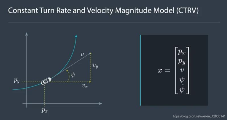
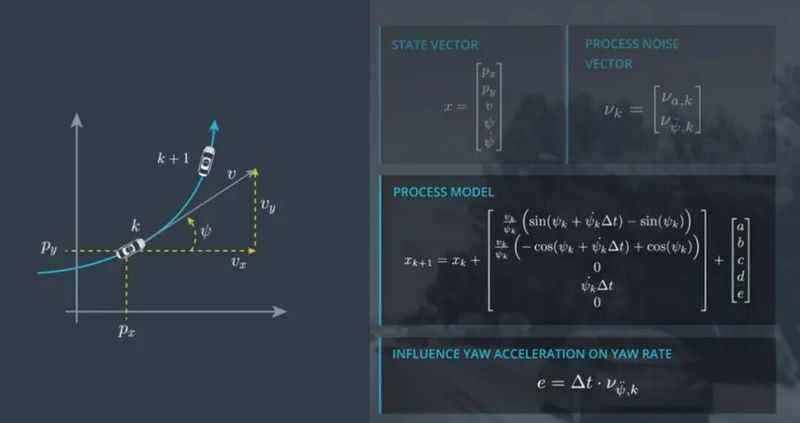
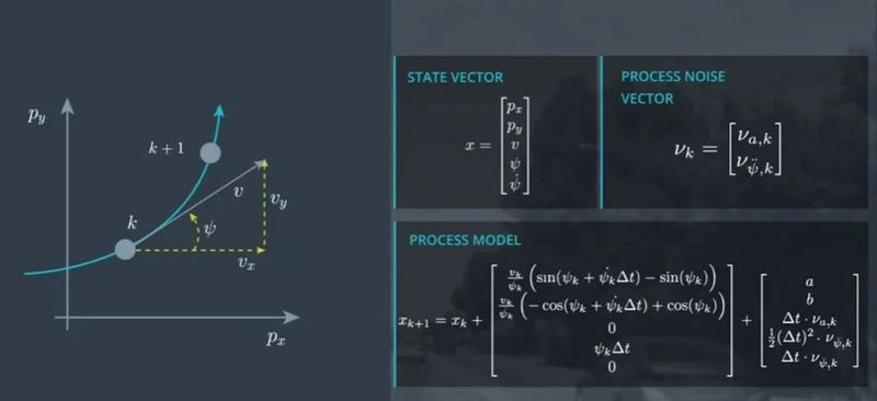
Constant rate and speed model (co)No, no, no, no
2. 1 target status of ctrv
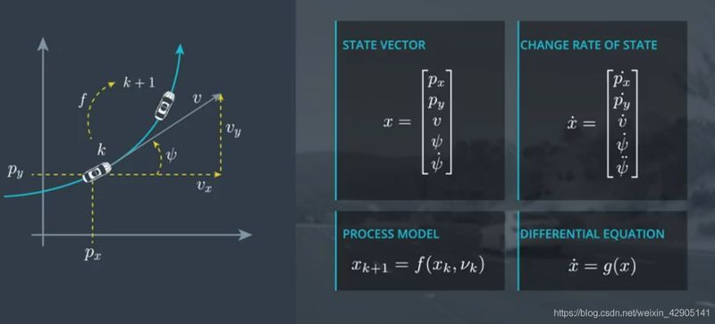
2. 2 ctrv status transfer function
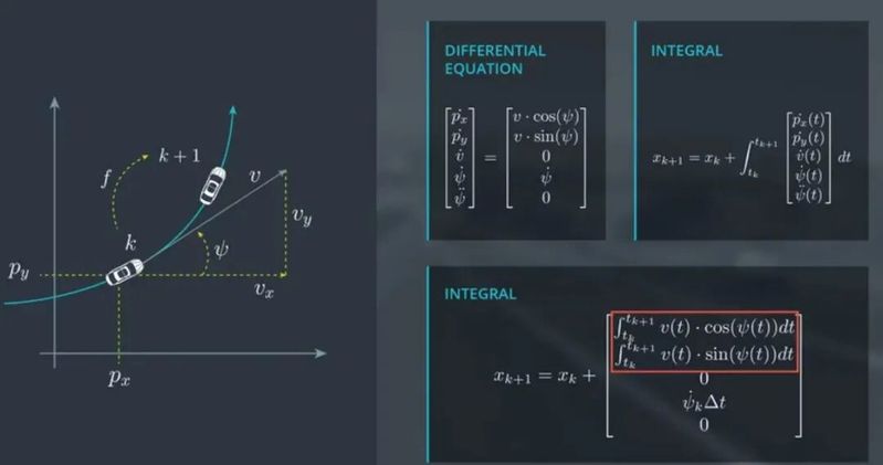
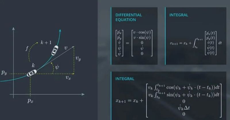
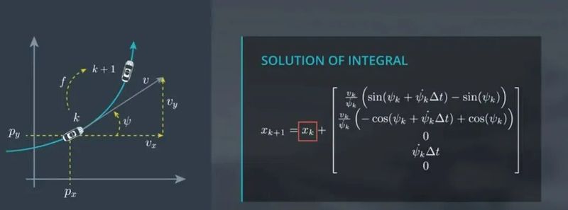
2. 3 ctrv access noise
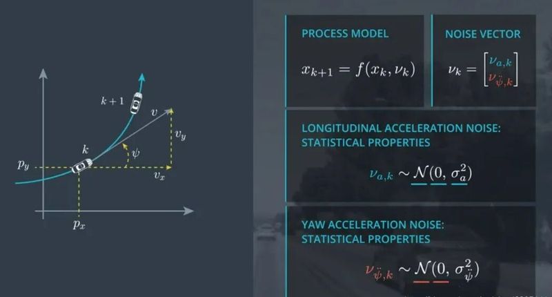
3. Predation
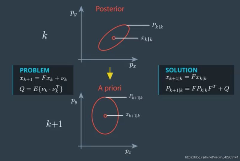
It is divided into three steps:
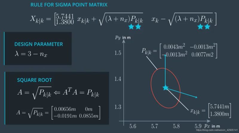
3. 1 general sigma points
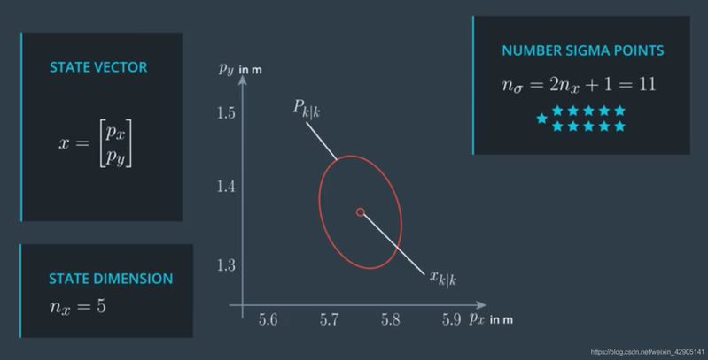
Normally, assuming the number of states is n, we create 2 n+1 sigma points, the first of which is the average of our current state μ, the average of sigma points is:

The zirconium is an ultra-parameter, according to the formula, the larger the sigma point, the smaller the sigma point, the closer it is。
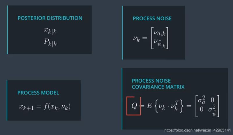
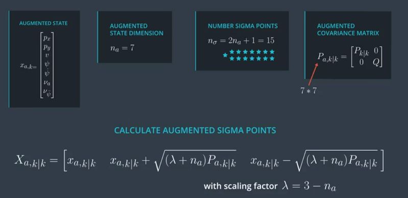
In our ctrv model, the number of states n includes, in addition to five, the treatment of noise mia and mitrometers, which also have non-linear effects on models. After increasing the impact of dealing with noise, our uncertainty matrix p became:

Among them, p's is our original uncertainty matrix (which is a 5x5 matrix in the ctrv model), and q is a coordinated matrix for addressing noise, which takes into account the form of a straight acceleration q in the ctrv model:
Calculating widening sigma points
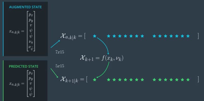
3. 2 projections

3. 3 projected averages and variance
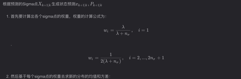
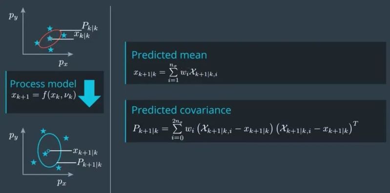
X k+1∣k is the weight of the sigma point for each state at each point, and the p's is the sum difference (uncertainty) for the a priori distribution pk + 1 ∣k is weighted by the difference for each sigma point。
4. Update
4. 1 predict mission
Puts the first map into the measurement space and calculates the average and the difference:
The measurements are divided into two parts, lida and radar, where the lida measurement model itself is linear, so our focus is on the treatment of radar measurement models, where the measurement non-linear map function is:
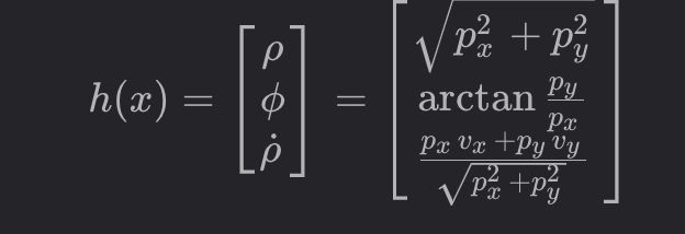
Measurement model, as shown:
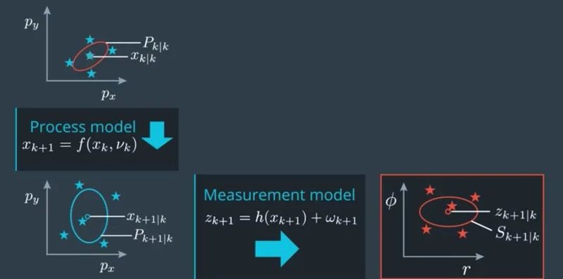
Once again, we use no-loss conversion, but here we can no longer produce sigma points, we can use the predicted sigma dots directly and we can ignore the noise part. The a priori non-linear map can then be expressed as the sigma point projection (i. E., the average and the agreement difference after the projection of the non-linear transformation):
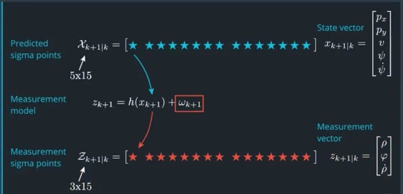
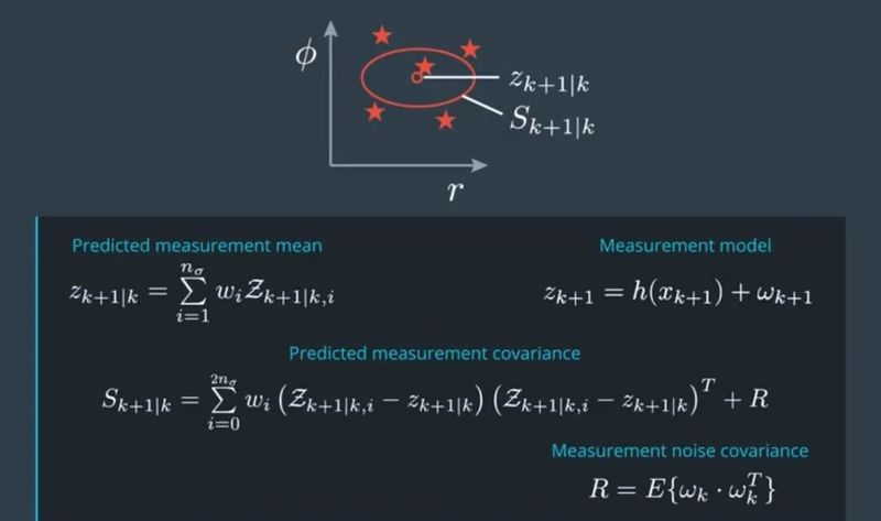
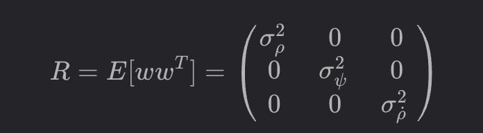
And here's r, which is also measuring noise, and here we're adding the synoptic difference in measuring noise directly to the synoptic difference because it has no non-linear effect on the system. In this case, for example, the radar measurements are:
4. 2 update state
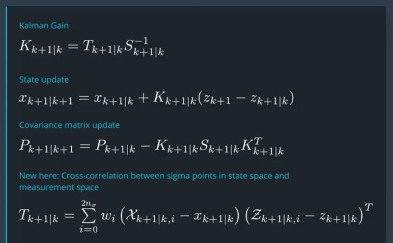
First calculate the interconnective function of sigma dot set in state space and measurement space tk + 1 ∣k t
Calculating kalman gain kk + 1 ∣
Updates the state to calculate $x k+1|k+ (where z k+1 is the new measurement, while z k+1∣k is the measure we calculated a priori in the measurement space)。
Update the status profile matrix, calculate pk + 1∣k + 1