


1 financial risk measures based on the theory of extremes and bayesian estimates [keywords of the paper] the theory of financial risk extremes: bayesmc [summaries of the paper] is used in this study to calculate financial risk values to help investors adjust risk models based on observational data and information to enable them to more accurately reflect the risk profile of financial markets and to make more sound investment decisions accordingly. In recent years, var and es have become widely used risk measurement methods in the financial community. Var (value atrisk), i. E. The greatest possible loss of the portfolio at a certain probability level for a given period of time. The advantage of var is that different market factors, risk sets in different markets, are one number that can accurately measure potential losses from different sources of risk and their interactions and adapt to the dynamic, complex and integrated trends of financial market development. But the var itself exists
Insufficient, i. E., the risk that the loss exceeds the value of var; and second, the risk measure is not consistent. Aitzner (1997) introduces the concept of an excepted shortfall (es), which measures losses beyond the loss expectancy of var, which is consistent with the risk measure. Most domestic investors are still investing directly in the stock market, and the volatility of individual shares is much greater than the volatility of the equity index. As a result, extreme var and es are of great interest for individual stock studies, and this paper attempts to use the pop model to estimate the var and es of individual shares in our stock market. 1 the var and es polar theory, based on the pot model, is a common method for measuring risk losses under extreme market conditions, with an estimation capability beyond sample data and an accurate description of the fractions at the end of the distribution, both for accurate calculations of var and es
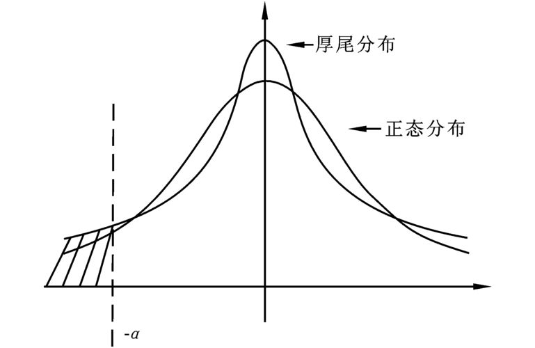
Three, very helpful. The pot (peaks over extreme) model is one of the most useful models in the polar theory, which models all sample data above a sufficient large threshold and therefore effectively uses limited extreme observations. This paper uses a pot model of parameters based on the broad paretto distribution, on which the corresponding fractions of the distribution of losses are estimated to calculate var and es. The normal gpd model parameter estimation method has a very similar estimation method, rectangular estimation and probability-weighted rectangular method. Existing studies have proved to be significantly more efficient under large sample conditions than other methods; rectangular estimates and probability-weighted rectangular methods are statistically calculated, but only for one-time periods. In addition, the var estimation method based on classical statistics is a backward-looking approach
4. The future loss is based solely on historical data and assumes that the past relationship between variables will remain unchanged in the future. It is clear that, in many cases, this is not consistent with actual experience, that the market will not necessarily repeat itself in the future, and that even if the observations are fully accurate, there is no guarantee that in the future something that has never occurred before, and that it is not surprising. Therefore, this paper uses a more effective approach, whereby bayes estimates that only the case of a representative thick tail distribution (>0) is discussed at this time >0, command, set, independent of each other, with the following a priori distribution, i. E., pareto(a, c) and gamma(a, b), of which a, c is the parameter of the pareto distribution, a, b is the parameter of the gamma distribution. According to the bayesian law, and the later distribution is as follows: f(,|x)l(x,)f()f(ii) of which, l(x|) is an approximation function, sample
This information follows the same approximation function into the estimation process. For the above posteriori distribution, it is not possible to estimate its parameters directly. For this purpose, e(x) and e(x) are calculated using the markov monte carlo simulation method (mcmc). The basic idea of mcmc is to simulate a sample path of the malkov chain, with the state space of the chain being the value of the estimated parameter, and the maximum distribution of the chain being the lateral distribution of the estimated parameter beyès. After full overlap, the malkov chain is constricted to a smooth distribution of targets rather than dependent on the original state. Filter the n status of the previous test period and the rest of the chain will be a sample of the target later distribution. The gibbs sample is the simplest and most widely applied mcmc method and is very convenient for practical application. The structures and mcmc simulations of the above posteriori distribution are based on a more mature software w inbugs. 2 empirical analysis of 2. 1 data describing my testimony
The bond market has undergone significant changes in the trading system for more than 10 years, particularly since the introduction of the rise and fall-off regime after 16 december 1996, which has been confirmed by a number of relevant research institutions in the country. Therefore, the closing price of the above-documented composite index (hci) from 16 december 1996 to 9 january 2007 is selected as the subject of the study to model the loss sequence of its rate of return. Basic statistical characteristics of shci: average -0. 000454 and standard deviation 0. 016543; deviation 0. 332547, with left bias; peak 8. 86027, > 3. So the distribution is biased and peaked. At the same time, its j-b statistical volume is 3103. 974, accompanied by a probability of zero, and the original assumption that distribution is normal is rejected. 2. The threshold of 2 is established in empirical evidence, usually in combination with qq figure
7. The threshold is determined by a map of the average excess function and a hill. As can be seen from the normal qq of shci and the index qq, the tail of shci is thick and the corresponding gpd model has shape parameters larger than zero. On the basis of the average excess function chart and the hillchart, we can make a preliminary estimate of the threshold, and on the basis of the crimer-von statistical volume w2 and the anderson-darling statistical volume a2 we can precisely get its threshold u = 0. 017833383, and the excess nu = 207 to make the gpd model. 2. The estimate of the 3 parameter winbugs is a program module for the establishment and analysis of the beyers probability model. Based on dialogue boxes and menu buttons, users are provided with an interface to analyse models using the marcov chain monte carlo methodology. We use this software to imitate the pot model. First take a sample from the condition later distribution

8. The parameters of the model are estimated with the available samples. In the analysis of the model, mcmc compulsive diagnostics are important and simulations must not be pre-repeated simply by a large number of iteratives. In the determination of mcmc composure, w inbugs can be judged by multi-layered iterative analysis of parameters, i. E. Input of multiple sets of initial values to form multi-layered interstellar chains, and when the parameter model is condensed, the iterative graphic results converge. The two sets of initial values entered into the model are presented in an iterative manner, followed by 2000 pre-repeats, and we can see in figure (2) the tracks of the two sets of initial values that form the two chains, as well as the convergence of the two chains in the condensed diagnostic maps, and the condensation of the diagnostic maps with one. As a result, 10,000 more gibbs are performed. The iterative values of w inbugs running from 2001 to 12,000 were estimated for model parametersb
9, ayes = 0. 3267, for comparison, we also give estimates of parameters based on a very semblance, mle = 0. 3146. 2. The estimates for the 4 polar var and es will be based on the estimated pot model parameters estimated by the bayes and mle into formula (6), and the estimates for the shci var and es at the corresponding level will be available. In table (1), both var and es values under the shci confidence level based on bayes ' estimate are greater than var and es values under the shci confidence level based on a very specious estimate, as the distribution parameter is considered by the bayes method as a random variable, which in effect increases uncertainty in the yield distribution of assets, and therefore the calculated risk value is greater than the value under the classic statistical estimate. The conclusion is that because of the rapid changes in financial markets, the longer the data are relevant to the current market situation, the less the early data can be used to illustrate historical issues and not at all to describe the current situation, where classical statistical methods rely too much on historical data to clearly guarantee the accuracy and validity of the var model. Using the bayes estimates to calculate var, the combination of experience and historical information with observations allows investors to adapt the var model to the empirical information available to them, with a view to obtaining var that more accurately reflects the risk profile of the market and makes the right investment decisions accordingly. Seven