The pid algorithms needed to be used to control the speed of the electrical circuits in the earlier period, since the concepts of previous studies had been blurred, so a loop of information had been searched online and retrained, although many were found to be text-based, with few examples showing the algorithm process. It's a record. It's an idea for new people to understand pid.
Purpose:
The importance of the pid should not be mentioned.
The purpose of this article is to show the algorithm process through an example and explain the following concepts:
(1) a brief description of what a pid is, why a pid, what a pid can do
(2) understanding the role of p (proportional link): the base ratio chain
Disadvantages: stable state error.
Question: what's a steady-state error.
(3) understanding i (corresponding) effect: eliminating steady-state errors ...
Shortcomings: increase in over-alignment
Question: how does the score eliminate the steady-state error?
(4) understanding the role of d (micro-points): increasing inertial response speed and decreasing overtones
Question: why can't it be reduced
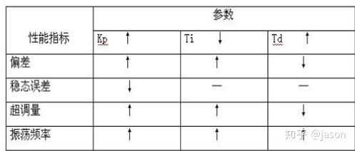
(5) understanding the role of the respective coefficients
Let's get down to business
I: what is a pid and why you need a pid
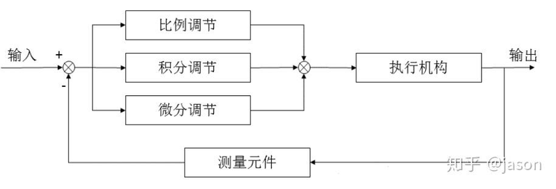
The following is the overall frame of the pid control, the process described as: set an output target, the feedback system returns the output value, and if it is inconsistent with the target, there is an error, and the pid adjusts the input value to this error until the output reaches the given value.
Question: so why do we need pids, like i control the temperature, i can't monitor the temperature, and the temperature stops as soon as it comes?
Here we have to start with our target, because all we have to do is to export what we can set, what kind of temperature change we want if we set a target temperature.
For example, the target temperature is set at 30 degrees, and the target is expected to reach figure 1 and it is expected to reach 30 degrees quickly and without shaking.
Then it should be understood that if the temperature stops at first sight, of course, if it's not too high, then it's not going to reach the level of figure 1, because the temperature will continue to rise after the temperature, and the temperature itself will spread through the air.
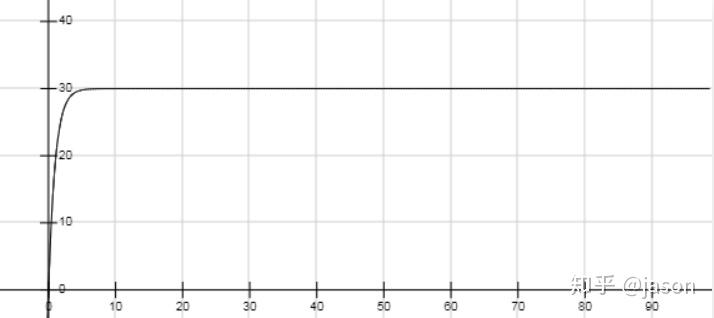
Figure 1 response targets for system output
The reason why we need pid is that ordinary controls can't get the output to a fixed value quickly.
If you throw that into question, let's start with a common example
Two, one example
Before we start, we need to move our formula out
Well, it's a pretty good formula. You know the basic definition of calculus and calculus. And ultimately, all our efforts are capable of understanding the formula, otherwise any fine metaphor can't really make you understand and use it.
Here we separate it
Kp - proportional constant
Ki = (kp*t)/ti - a factor constant
Kd=(kp*td)/t - - breeze constant
Here's one example of how this equation works.
(1) ming has been given a task: there is a bucket that needs to remain at 1 m altitude at all times, and there is currently 0. 2 m water in the bucket
So ming uses the p-scale method to add water: an error of 1 m per measure and add the amount of water proportional to the error
For example, kp = 0. 5.
For the first time, the error was 1-0. 2 = 0. 8 m, so the amount of water added was kp*0. 8 = 0. 4 mm.
Second, the error is 1-0. 4 = 0. 6 m
We find this perfect, and the scale will solve the problem perfectly, but wait, before we do this, we're looking at ming's new mission
(2) ming's new mission: there's a bucket, but there's a hole in the bottom of the bucket, and there's still a 1 m height, and there's currently 0. 2 m of water in the bucket, but every time you add it, it's going to run out of 0. 1 m. This example is close to an example of what we actually do, such as resistance to electric friction, loss.
Let's get ming to work,
For the first time, use of p (scale control) u = kp* e
Kp = 0. 5
L (final level) = current input u plus last level
First, the error is 1-0. 2 = 0. 8 m, so the amount of water added is kp*0. 8 = 0. 4 mm. The final water level is 0. 4 + 0. 2-0. 1 = 0. 5
Second, the error is 1-0. 5 = 0. 5 mm
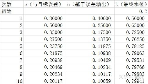
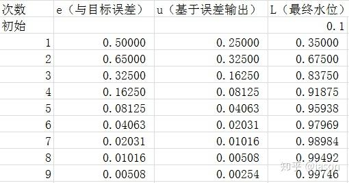
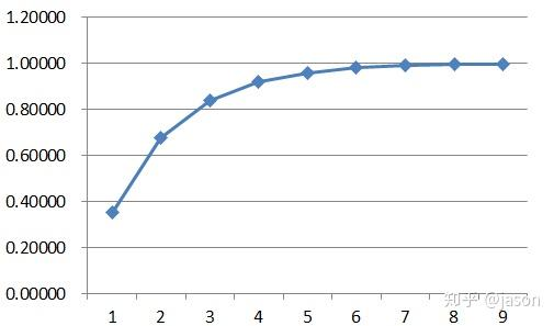
Table 1
We found a problem, and the water level was finally stabilized at 0. 8m, and it's understandable that when the error was 0. 2m, 0. 1 when the water was added, each time it was inserted, it was just missing.
Here, the concept of steady-state error is introduced: the error of the system when it reaches a steady-state.
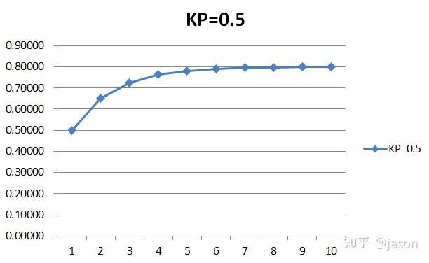
Then let's increase the kp.
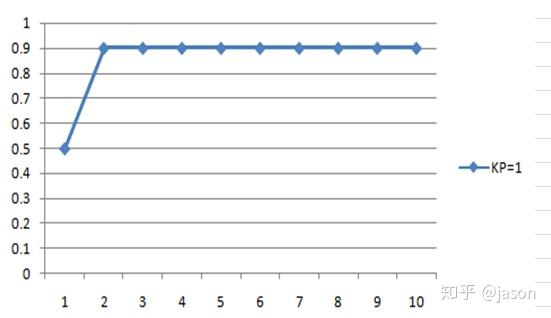
We've found that the error is getting smaller, so let's keep it growing
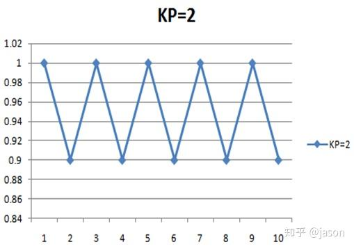
We found the system is shaking.
This is an excel circuit where you can adjust parameters to observe changes
Conclusion: proportional controls introduce steady-state errors that cannot be eliminated. ... An increase in the ratio constant can reduce stable-state-specific errors, but if too large they cause systemic shocks and instability.
In order to eliminate the steady-state error, add a second score using pi u = kp*e+ki*sum n=k}e(k)}
The factor control is to add up all historical errors and multiply them by a factor constant.
What's that supposed to mean.
Or should i start with kp = 0. 5, ki = 0. 3
First: error of 0. 8, proportional of kp*0. 8 = 0. 4, integral of ki*(e) = 0. 24, adding u 0. 4 + 0. 24 = 0. 64. Final water level 0. 2 + 0. 64-0. 1 = 0. 74 m
Second: error of 0. 26, ratio of kp0. 26 = 0. 13, integral kp* (e(1) + e(2)) = 0. 318, adding u 0. 13 + 0. 318 = 0. 448 final water level 0. 74 + 0. 448-0. 1 = 1. 088 m
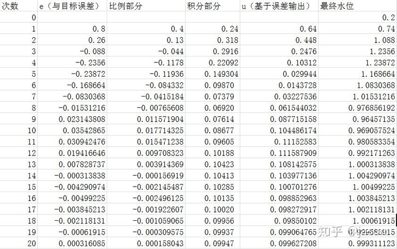
Table 2
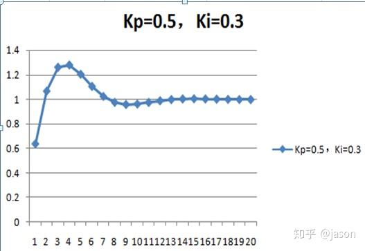
We found out that, although the process was a twist, it could eventually stabilize to a set value.
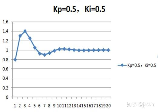
What if it's bigger than ki
This is an excel circuit where you can adjust parameters to observe changes
Conclusions
As long as there's a deviation, the points accumulate until the error is zero, and the sequence is no longer cumulative and becomes a constant that offsets the steady-state error.
As you can see in table 2, when the system stabilizes, it's about 0. 1.
2 the introduction of points eliminates steady-state errors, but increases the ultra-module, and ki increases and increases the ultra-module.
In order to eliminate the hyperbolicity, we introduced a differential effect
Now the formula becomes u = kp*e+\sum n 0}e(k)}+kd(e)-e(k-1)
Kp = 0. 5, ki = 0. 5, kd = 0. 3
First: error of 0. 8, ratio of kp*0. 8 = 0. 4, score of ki* (e(1)) = 0. 24, calculus = 0 (because the pre-water level difference is 0. 8)
Second: error of 0. 1, kp* 0. 1 = 0. 5, kp* (e (1) + e(2)) = 0. 45, calibrated of kd* (e (2) - e(1)) adding u 0. 5 + 0. 45 - 0. 21 = 0. 29. Final water level 0. 9 + 0. 29 - 0. 1 = 1. 09 m
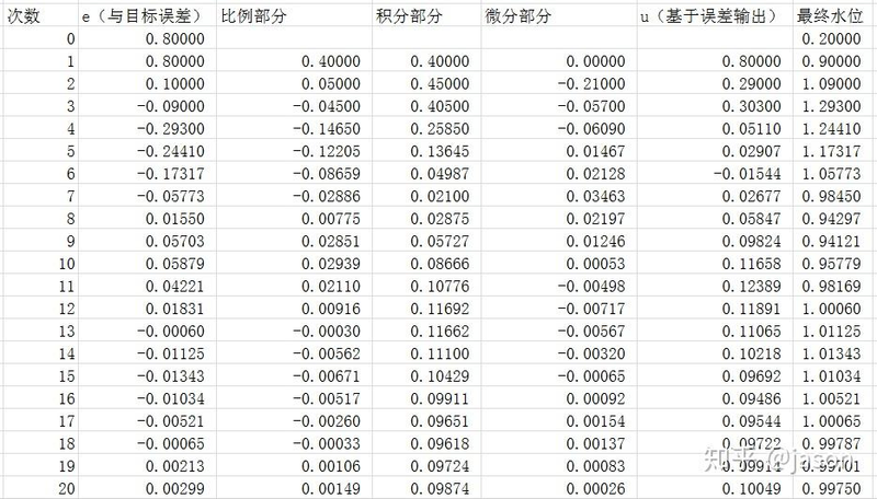
Table 3
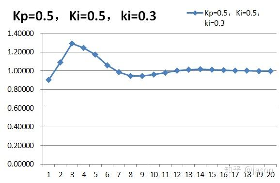
And we found a comparison between the kp = 0. 5 and the ki = 0. 5, and the shock of this graph is reduced, and that's precisely what happened with the calculus,
As you can see in table 3, when the second error was 0. 1, the last error was 0. 8, the calculus was a negative, preventing the result from changing fast.
Conclusions: calibration reduces the trend of overtones.
But this wave shape is still convulsing, yes, and don't forget, it's a value that i set, and we can't expect us to set a value that makes the pid work perfectly, and if you simulate it with excel, you'll find that if ki, kd, is set up bigger, the system will shock.
So we're going to have to fix kp, ki, kd, and actually try to get the output up to the requirements of figure 1
Of course, this example actually uses the pi, and we're here to understand how it works.
If there's anything wrong, please indicate it in time.